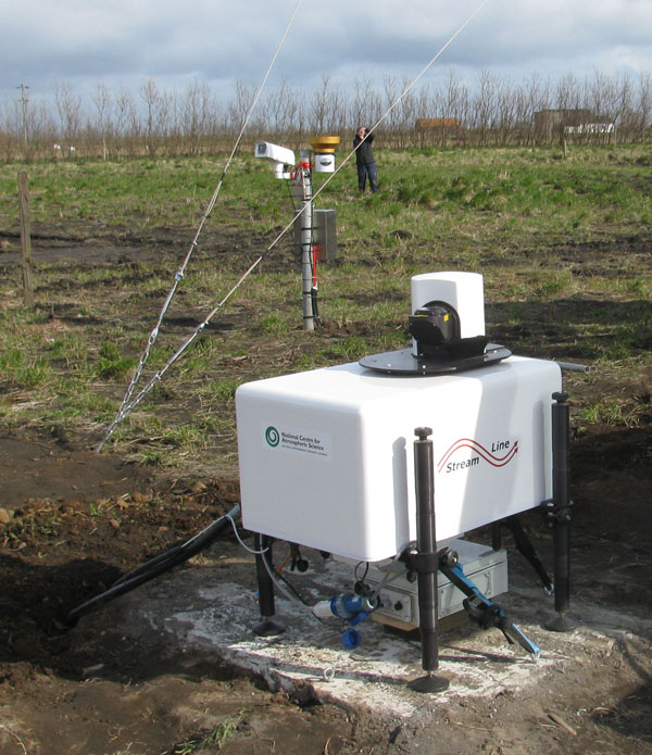
Doppler Aerosol Lidar

The following is a brief introduction to the background science of how the instrument works and a brief discussion of how the data the instrument produces can be interpreted.

1. Scattering of light

Scattering of electromagnetic (EM) waves by any system is related to the heterogeneity of that system: heterogeneity on the molecular scale or on the scale of aggregations of many molecules. Regardless of the type of heterogeneity, the underlying physics of scattering is the same for all systems.

Matter is composed of discreet electric charges: electron, protons. If an obstacle, which could be a single electron, an atom or molecule, a solid or liquid particle, is illuminated by an EM wave, electric charges in the obstacle are set into oscillatory motion by the electric field of the incident wave. Accelerated electric charges radiate EM energy in all directions: it is this secondary radiation that is called the radiation scattered by the obstacle. In addition to reradiating EM energy, the excited elementary charges may transform part of the incident EM energy into other forms (thermal energy for example), a process called absorption.

Everything except a vacuum is heterogeneous in some sense. Even in media that would usually be considered to be homogeneous (pure gases, liquids or solids), it is possible to distinguish between different heterogeneities if you have a fine enough probe: therefore all media scatter light. Scattering can be either:

Elastic: wavelength of the EM radiation is conserved.

In-Elastic: wavelength of the EM radiation is NOT conserved.
As an illustration, imagine throwing a white ball at a wall: if the ball comes back white the scattering was elastic, it comes back a different colour it was in-elastic.

The intensity of scattered light at any point around the scattering body is determined by the wavelength of the light illuminating the body, the size of the body, the composition of the body and the shape of the body. The composition of the body is reflected in the refractive index of the scatterer and it is complex: the real part indicating the body’s ability to scatter the incident light and the imaginary part the degree to which the body absorbs the light. The direction into which light is scattered is usually referred to as FORWARD scattered: light scattered in the direction of illumination, BACKSCATTER: light scattered back along the line of transmission to the source, SIDESCATTER: light scattered to the side.

The shape and homogeneity of the scattering body composition also have an effect on the polarisation of the scattered light. The electric field vector of an electromagnetic wave at any instant in time displays some orientation in space and this orientation can be fixed (linearly polarised), or rotating with time (circularly or elliptically polarised). Changes in the orientation of the electric field vector occurring on when the light is scattered is termed depolarisation and is predominantly caused by internal reflections. For a purely spherical body that is homogeneous in composition backscattered light is polarised in the same plane of polarisation as the incident light. The degree of depolarisation depends on the amount and complexity of the body’s deviation from sphericity, homogeneity of refractive index and relative size of the contribution to the refractive index of absorption: backscatter depolarisation is confined to particles that are not overwhelmingly absorbing.

2. LiDAR

A LiDAR (Light Detection And Ranging) is an optical instrument that comprises a transmitter to project pulses of light into the atmosphere, a telescope to collect the light scattered, and some electronics to analyse the intensity of the scattered light collected. Such systems can be arranged such that the transmission and collection units are physically separated (bi-static) or co-located (mono-static). For mono-static systems, the local arrangement of the transmission and collection elements can also vary with either the transmitter alongside the telescope or transmission is through the telescope. The latter arrangement is the case for the HALO LiDAR.

The HALO LiDAR uses light with a wavelength of 1.55 μm. As the intensity of the light scattered is greatest when the scattering body is similar in size to the incident radiation this instrument “sees” the aerosol rather than the molecular components of the atmosphere. In addition to applying a mathematical retrieval algorithm to intensity profile measured in order to retrieve the Aerosol Backscatter Coefficient (β), the velocity at which the aerosol is moving along the beam is also determined using the Doppler effect – this is termed the radial velocity. Usually, the sign convention for Doppler analysis is that +’ve is towards the observer and -‘ve away, however for this system the meteorological convention of +’ve away (or up) and –‘ve towards or down is used. The ability to measure radial velocity coupled with the instrument’s movable head means profiles of horizontal wind speed and direction can be determined.

This Lidar also applies the same β retrieval algorithm to the light scattered and polarised at an angle of 90° to the transmitted light: this is the cross channel and the ratio of the β from the cross channel to the total β gives the depolarisation ratio δ. How the β from the two channels varies can provide a great deal of information about clouds.

Water clouds: The scattering bodies in this type of cloud are usually spherical and compositionally homogeneous and as such the backscattered light would be expected to undergo no depolarization, however, a depolarised signal is often observed. As the light penetrates the cloud and the cloud droplet concentration increases and scattering of near-backward rays into the LiDAR field of view occurs. It is only the truly backscattered ray that does not undergo depolarisation and these near-backward rays have some degree of depolarization so when light scattered into the LiDAR field of view a signal in the cross channel is detected. This parasitic signal increases as the cloud droplet size increases, with the depth of penetration and with cloud droplet concentration.

Ice clouds: δ for randomly orientated ice crystals increases as axis ratio increases: that is, a the crystal habit changes from plate to column but even a thin plate ice crystal will cause a substantial depolarised signal in comparison to other atmospheric targets. Using ray tracing theoretical values for δ can be determined, for example:

Thin Plate: 0.339
Plate: 0.355
Thick Plate: 0.394
Short column: 0.362
Column: 0.550
Long Column: 0.563

Mixed phase clouds: the use of depolarisation can allow for the identification of regions in a cloud of different phase (water or ice) and the zones of transition between them, however this is restricted by optically dense clouds where the light can only penetrate a few 100 m. It can be used to detect ice virga and the transitional zone for light precipitation.

Precipitation: snow, hail, graupel, rain (from melting ice), and rain/drizzle (formed by coalescence) can all be distinguished. Snow and other rimmed particles give rise to large δ due to the complex shape and a large number of scattering planes. Even raindrops give rise to a depolarization signal due to their departure from the spherical as they fall, an effect that increases with increasing size: drizzle is small and almost spherical hence δ ~ 0, but typical millimeter size rain will induce some sort of δ response. Significant δs can also be induced in water droplets by collisions as this causes droplets to oscillate: the shape changes.

The system is fully networkable and can be installed on most networks: it also has a second network interface for direct connection to a computer. Access on either port is via VNC and is password protected: users will be issued with a password when taking delivery of the instrument.

An internal GPS provides the option of time synchronisation for the onboard PC. By default, this is activated but users can request that this be deactivated and the clock synced to a network time server. It is advised that the LiDAR PC is time synched at regular intervals.

The GPS also provides height and positional information but note that this is not logged by the system: if operating on a moving platform an external source for position and height will be required.

The system also has internal tilt sensors to aid in levelling the instrument when deploying: these are not logged.

This instrument needs no special licence to operate.

Operation using the depolarisation channel

The optical arrangement within the instrument scanning head that passes the light to the co-planar and cross-planar electronics means that:

Depole is only available when the instrument is operating in stare mode

When in stare mode and depole is selected the azimuth position selected by the user will be overwritten and the head will reposition to an azimuth of 310°

Operation in cold and hot climates

Operation in cold climate: The instrument does have an extended operational temperature range however it should be noted that the signal amplifiers will only operate reliably above an instrument internal temperature of 15°C. The system is well insulated and the temperature is actively controlled to stay at 25°C but it is recommended that you ensure the instrument is deployed ‘warm’; that is, it has been operated and allowed to reach a stable ‘warm’ temperature. Should it be deployed cold the signal amplifiers will appear to be operating but will not actually be sensing.

Operating in a hot climate: Should the active cooling be unable to sustain the internal temperature of the instrument below 40°C the system will automatically shutdown.

While every effort has been made by the manufacturer to provide accurate and calibrated data products, HALO Photonics does not currently guarantee the calibration of the data in absolute terms. Wherever and whenever possible instrument comparisons take place where, for example, wind profiles derived from a range of measurement sources are compared. It is the results of such comparison exercises together with continual monitoring both during and after a deployment, and the system diagnostics that allows the instrument scientist to determine if the system is operating optimally or requires manufacturer servicing and intervention.

Consumables

• The user will need to supply both power and networking cables.
  • Network
    • requires to be terminated at the instrument end by a Bulgin Buccaneer IP68Cat5e RJ45 connector.
  • Power
    • requires a 16A 240V 3P connector at the instrument end.
• The user will also need to supply their own PC\laptop system from which they can connect to the LiDAR: this will need to have a VNC viewer installed.

Costs:

• Instrument Insurance
  • This system must be insured by the user for £190K and covers loss, theft or damage to the instrument: damage is that over and above general wear and tear. The system has been designed to be rugged and autonomous. Even so, the end-user must respect the fact that the system is a precision optical instrument that must be treated with great care.
  • The user is responsible for the instrument from the time it leaves AMOF to the time it is returned and signed off as in an acceptable operating condition by the IS: this will be done as soon as is possible on its return.
• Public Liability Insurance
  • We are not liable for any damage or injury arising from the deployment or operation of this instrument when unattended by the instrument scientist.
• Shipping Expenses
  • The user is liable for all costs arising from the shipping of the instrument both to and from a deployment.
• IS T&S
  • The user is responsible for coving the travel and subsistence expenses of the IS while attending the instrument.

Shipping:

The system when packed ready for shipping consists of a single flight case that sits on a separate dolly of which two of the wheels have breaks. The case contains the LiDAR, and its power supply comprising a UPS and AC/DC convertor in separate IP65 enclosures.

Shipping dimensions: 112 cm (L) x 70 cm (D) x 120 cm (H)
Shipping weight: 163 kg

The LiDAR should be deployed on a surface that is not liable to get excessively hot, as the cooling aggregate (air-flowed heat exchanger) is located on the underside of the base unit. Steps should be taken to minimise the heat generated underneath the LiDAR from direct sunlight – a turfed area is ideal. For cold running, a windbreak to protect the LiDAR from the prevailing wind will help.

When considering the deployment locations some thought needs to be given to potential obstructions to the beam. This will also depend very much on how the instrument is to be operated but in general, an unobstructed full-sky view is recommended.

Although requiring two people to move, the system will require securing to a surface to prevent movement due to wind impact. It should also be located on a secure site to avoid theft and vandalism.

For ease of operation, it is advised to ensure that there is network infrastructure to hang the instrument on. If a network is not available then the user will have to connect to the instrument via the local network connection using a cross-over cable.

At sites where animal activity is likely precautions will need to be taken to prevent chewing\pecking of cables.

Eye safety

• This system contains a class 1M category laser and is eye-safe for all conditions of use.

Manual handling

• When in its packing case it is recommended that four people be used when lifting. Once out of the case the instrument requires two people to lift and or move it. At least one cable has to run to the instrument and so users should be aware that both the instrument and the power cable constitute a trip hazard and users should take appropriate actions to minimise this.

Electric safety

• Under no circumstances should any attempt be made to open the main body of the instrument. The power supply and UPS units that are separate to the instrument can be opened if problems occur but only once they have been disconnected from both the supply and the instrument. Only appropriately qualified persons should attempt to fault find these units.

Attended operation

• There is no requirement for the system to be attended during operation from a safety standpoint.

When unpacked and deployed the LiDAR has the following physical characteristics:

Foot print: 150 cm (L) x 100 cm (W) x 150 cm (H)
Weight (not including shipping case): ~80 kg
Power: 300W @ 240VAC
Operation temperature: -20°C to 40°C

Cable power: The user will need to supply a 3 core power cable of appropriate length for the deployment. This need to be terminated by a 16A 240V 3P (2P + E) connector at the instrument end.

Cable signal: The user will need to supply either
a standard cat5 ethernet cable of appropriate length for the deployment, or a cat5 cross-over ethernet cable of appropriate length for the deployment

The default output of the LiDAR is range corrected retrievals of aerosol backscatter coefficient and radial wind speed at user-specified azimuth and elevation angles.

An option is to operate the instrument to generate profiles of mean wind speed and direction. In this case the data is presented in terms of height above the instrument.

The usual convention for Doppler motion is with the +’ve direction being defined as towards the instrument: the opposite to that in a meteorological application where the +’ve direction in upward: that is away from the instrument. Irrespective of the elevation angle all the data termed ‘radial wind’ uses the direction convention:

• +’ve AWAY from the instrument
• -‘ve TOWARDS the instrument

that is it follows the meteorological convention.

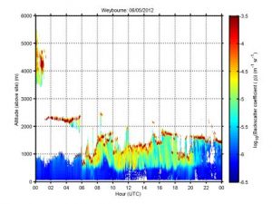
Backscatter coefficient

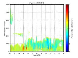
Radial Winds – when vertically pointing as in this example, radial winds are equivalent to vertical winds (the +’ve direction being away from the instrument that upward.)

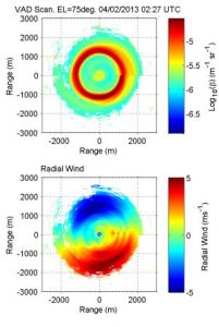
Backscatter and radial wind field for a volume scan: that is azimuth angle scans through 360° at a fixed elevation angle.

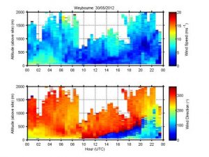
Mean wind speed and direction profiles for a 24hr period. Profile measured every 10 minutes.

Field Data

• The instrument produces a range of out files and all are text format.
• The user can download (but not delete) this data from the instrument but it should be noted that this data will not have been quality controlled.

Archive Data

• Data is provided in NetCDF files following the AMOF data standard
• Files contain no more than 24hr of data.
• Instrument name is
  • ncas-lidar-dop-1
• The data product(s) associated with this instrument:
  • v1.1
    • Vertical dimension uses “index”.
    • For profiling instruments (not the radiosondes) the altitude variable and profile variables have dimensions of time and index
    • The version should be used if the altitude variable is likely to vary over the duration of the file.
    • mean-winds-profile
    • aerosol-backscatter-radial-winds
    • depolarisation-ratio
  • v2.0
    • Vertical dimension uses “altitude”.
    • For profiling instruments (not the radiosondes) the altitude variable has dimensions of altitude and the profile variables have dimensions of time and altitude
    • The version should be used if the altitude variable does not vary over the duration of the file.
    • mean-winds-profile
    • aerosol-backscatter-radial-winds
    • depolarisation-ratio
  • Example data file
    • How to use example data
    • v1.1
      • ncas-lidar-dop-1_ral_29001225_aerosol-backscatter-radial-winds_fixed_co_standard_v0.1.nc
      • ncas-lidar-dop-1_ral_29001225_mean-winds-profile_v0.1.nc
      • ncas-lidar-dop-1_ral_29001225_depolarisation-ratio_standard_v0.1.nc
    • v2.0
      • ncas-lidar-dop-1_ral_29001225_aerosol-backscatter-radial-winds_fixed_co_standard_v0.1.nc
      • ncas-lidar-dop-1_ral_29001225_mean-winds-profile_v0.1.nc
      • ncas-lidar-dop-1_ral_29001225_depolarisation-ratio_standard_v0.1.nc